Specialized Loss Functions for Regression
Normally, when performing regression to fit an analytical function to data, there are only a couple standard “textbook” methods to follow. The first is a least-squares fit, usually solved via gradient descent or matrix methods. The other is single-class SVM. This article will discuss a variant on the least-squares method by exploring different loss functions and the resulting behavior.
Let us begin by identifying function candidates. I find it useful to think of these functions as potential wells; it provides a good physical intuition and my descriptions will reflect this viewpoint. Optimization then will seek to find the lowest-energy state. Least-squares provides a basic parabola, with the lowest energy state at 0 and an increasingly steep gradient further from the origin. This form provides self scaling behavior ( f[2 x] == 4 f[x] ) and optimization of this function results in a global minimum. These are useful properties, but the increasing gradient at larger values also means a fit is affected strongly by outliers. This behavior is shared with single-class SVMs, whose result is determined solely by outliers. There are other methods to address this problem, but in this article we will discuss changing out the loss function for another potential well.
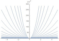
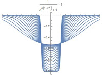
Quadratic Well (Least Squares)
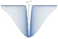
The first two functions are based on the Gaussian function and a rational function. I will refer to the second as the “reciprocal well”. Both have similar properties, and have a scale parameter which scales the width of the well. They are steep in the center and plateau quickly away from the origin.
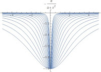
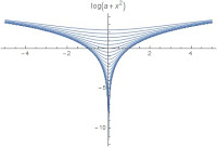
The next two are based on the Logarithm and Logistic functions. I will refer to the second as the “square well”. They have distinct shapes, with independent shape and width parameters. The logarithmic well does not plateau at any value, and thus is less sensitive to local optimality effects as the others. The square well is notably flat near the origin as well as at large values.
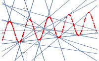
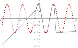
Local Optima
Now that we’ve introduced the well functions, let us explore the properties. The most notable property of each is existence of many local optima. Linear regression against a curved function will result in a closer fit to parts of the curve, “snapping” to curve tangents and preferring close fits to local regions. We can demonstrate this by fitting a linear regression against a sinewave function using a variety of starting values. As can be seen in this graph, the resulting lines find areas with multiple tangents or the longer, flatter single tangents. Similar results are achieved with each well function.
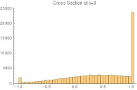
These well functions differ notably when used to fit data sets with structured uncertainty. The example given is a truncated Gaussian distribution along a linear band; data points are strictly bounded within y=x+/-1, and within that band the distribution is concentrated slightly above the center. Concentrated regions exist on the upper and lower edges of the band.
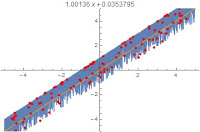
A traditional least-squares fit results in a line close to the central peak of the band. A Gaussian or reciprocal well results in a fit on the upper edge of the band, where the distribution is most concentrated. A square well with appropriate width and shape parameters will result in a fit along the geometric center of the band, with an intercept close to the origin.
I hope you found this brief overview interesting. The complete notebook detailing this research can be downloaded here in pdf format. I began researching this as a component of a modeling idea similar to a hybrid between decision trees and neural networks… Hopefully, I will have something to write about on that front in the near future. Until then, Happy Computing!
UPDATE:
I have gotten a prototype regression tree working which uses this type of regression with a recursive divide-and-conquer approach to produce an analytical function fit. An example tree, fit against a sinewave function, is shown below. The tree depth is 4, and it is similar to a piece-wise linear fit:
The function is fairly complex, but purely analytical, as is the process the produced it:
This is a very simple example of a process I am working on generalizing to multiple dimensions, more complex forms, and to fit inside neural network frameworks. A pdf export of a notebook detailing this tree regression can be downloaded here.